Spatial machine-learning model diagnostics

When applying machine-learning models to geospatial analysis problems, we still rely on non-spatial diagnostic tools for model assessment and interpretation.

In model assessment, spatial cross-validation has been established as an estimation techniques that determines the transferability of a model to similar nearby areas. Nevertheless, it does express how a model’s predictive performance deteriorates with prediction distance. In model interpretation, permutation-based variable importance is an intuitive and widely used technique that estimates the contribution of individual predictors or groups of predictors to a model’s predictions (see, e.g., Molnar 2019). However, it does not reveal if and how a variable is more relevant at shorter or longer distances.

My recent contribution (Brenning 2023) proposes novel spatial diagnostic tools that address these issues:

When using SPEPs and SVIPs to compare difference machine-learning and geostatistical models, they indicate which models are better at interpolating and extrapolating at different prediction horizons, and which predictors they are able to exploit.

How it works

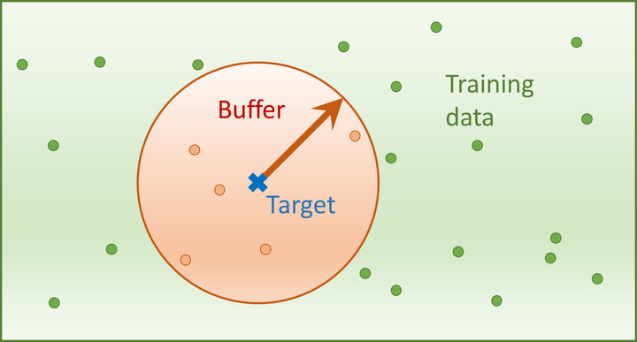
SPEPs aim to find out how well a model predicts at a given prediction distance. To estimate this performance, we leave out one observation at a time from the training set. We can enforce a particular prediction distance by removing from the training sample all data that falls within that distance around the left-out data point (see buffer zone in the figure above). We train our model on the remaining data, and estimate its error on the left-out point. This is repeated for each observation in our dataset, and the prediction distance is furthermore varied from 0 to some upper limit that depends on the size of the study area. Aggregating these results gives us a distance-dependent curve, the spatial prediction error profile (SPEP).

Unlike the kriging variance, which is only available for this specific geostatistical method and requires certain assumptions to be satisfied, the SPEP technique is model-agnostic, which means that it can be applied to any model – statistical, geostatistical, or machine learning.

In general, permutation-based variable importance is based on measuring how much a model’s predictive performance deteriorates when a predictor variable is permuted, or “scrambled.” We can do this also in the estimation of SPEPs, which will indicate how strongly the predictive performance at different prediction distances relies on a given predictor. I refer to this as the spatial variable importance profile (SVIP).

SPEPs and SVIPs can be applied to interpolation, regression, and classification problems in the spatial domain. Here we will have a brief look at a well-known dataset that is often used to introduce geostatistics, but in the paper I also demonstrate their application to a classical remotely-sensed land cover classification problem (Brenning 2023).

Case study: the Meuse dataset

The Meuse dataset characterizes topsoil heavy-metal concentration on a floodplain in the Netherlands. The logarithm of zinc concentration (logZn) can be modeled based on elevation (elev), the (square root of the) distance to the river (sqrt.dist), and the x and y coordinates; I will use regression methods such as random forest (RF) and multiple linear regression for this (MLR).

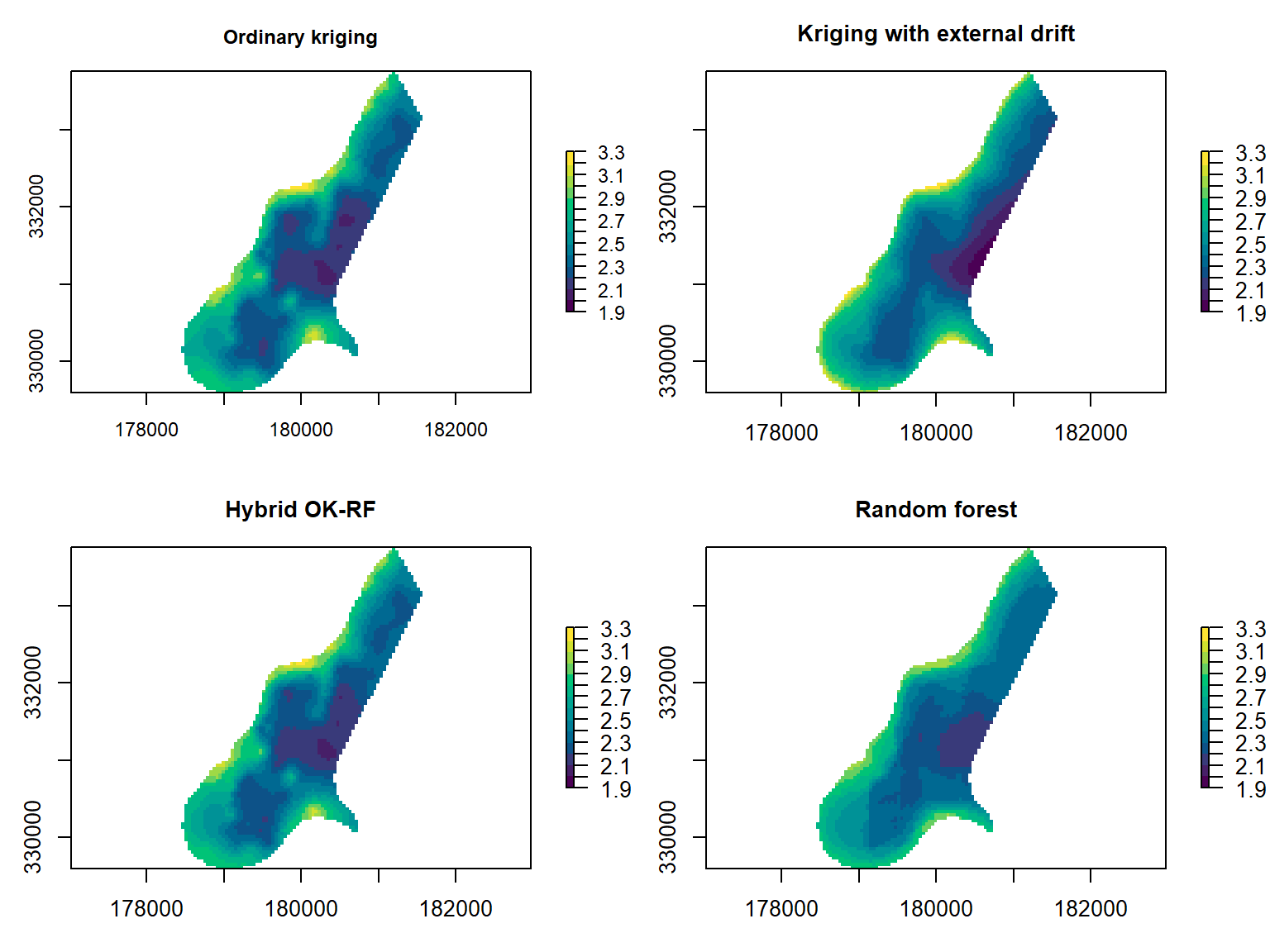
Figure 1: Spatial prediction maps of ordinary kriging (OK), kriging with external drift (KED), random forest (RF), and a hybrid OK–RF method.

Due to the strong autocorrelation at short distances, it is also possible to use interpolation methods such as ordinary kriging (OK) or nearest-neighbour (NN) interpolation, which I also include in my comparison. Hybrid methods are therefore also appealing – here I use kriging with external drift (KED) and also a combined OK–RF technique that blends OK into RF as the prediction distance increases.

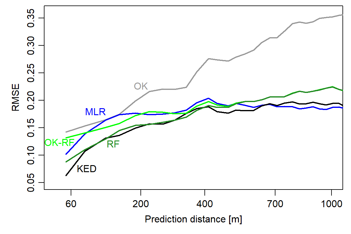
Figure 2: Spatial prediction error profiles (SPEPs) of the geostatistical, machine-learning, and hybrid models.

This is what we can learn from the SPEPs:

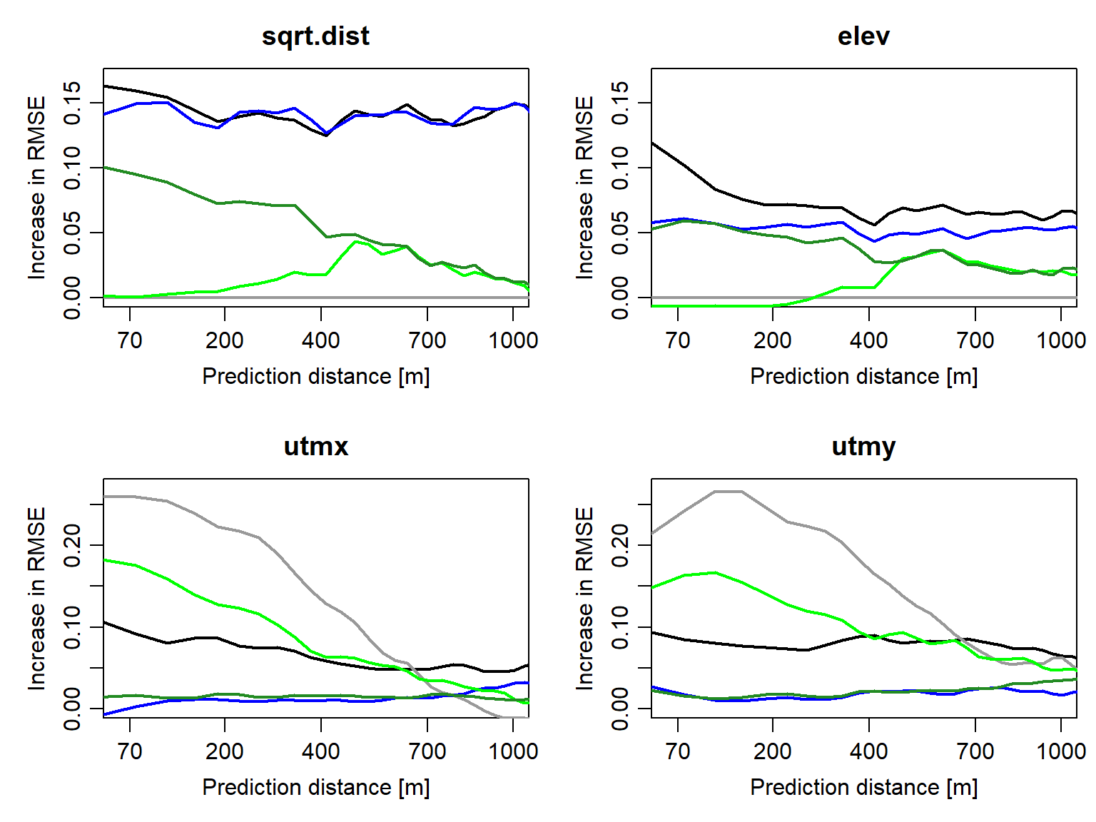
Figure 3: Spatial variable importance profiles of the predictor variables for OK (grey), KED (black), MLR (blue), RF (dark green), and hybrid OK–RF (light green).

The SVIP confirm the expected differences between interpolation, regression, and hybrid models: Interpolation models only rely on x and y coordinate information, which becomes less useful at greater distances. Regression models, in contrast, only rely on predictor variables, and their importance may decrease with distance (see RF, KED). SVIPs detect the ability of the hybrid OK–RF model to exploit proximity information (i.e., coordinates) at short prediction distances, while ramping up the importance of predictor variables at greater distances.

Conclusion

SPEPs and SVIPs are effectively able to visualize how model performance and variable importance vary with prediction distance. They are therefore valuable additions to our diagnostic toolkit for spatial modeling.

R Code

The R code for this analysis is available in a Github repository. It will be migrated into the sperrorest package, adding functions for computing and plotting spatial prediction error profiles (SPEPs) and spatial variable importance profiles (SVIPs).

References

Brenning, A. 2023. “Spatial Machine-Learning Model Diagnostics: A Model-Agnostic Distance-Based Approach.” International Journal of Geographical Information Science 37: 584–606. https://doi.org/10.1080/13658816.2022.2131789.
Molnar, C. 2019. Interpretable Machine Learning: A Guide for Making Black Box Models Explainable. https://christophm.github.io/interpretable-ml-book/.