How to encode slope aspect (and other cyclic variables) in environmental ML models
Slope aspect is a standard ingredient of statistical and machine-learning models of Earth surface processes and topoclimatic variables, and in digital soil mapping and ecological modeling (e.g., Brenning et al. 2015; Deluigi, Lambiel, and Kanevski 2017). But unlike other quantitative predictors, it’s a strange beast:
- The distance between 359° and 1° is 2°, not 358°.
- Is 180° greater or smaller than 0° (=360°), or can it be both?
- Two times 180° is 0° (or at least equivalent to 0°).
Unfortunately, all statistical and ML models apply at least one of these concepts - distance (or subtraction), order, and multiplication (and addition) to their predictor variables, including slope aspect.
You’ll also realize that the same thing happens with other cyclic and directional variables such as the time of the day (London 2016), or the strike and dip of geological strata.
Yes, we do. Or we might. Let’s take a closer look at it to see how bad it might get. We’ll apply four statistical and ML techniques to a simulated dataset to compare the following strategies:
- Direct encoding: Slope aspect as an ordinary, untransformed predictor (Meyer et al. 2019);
- Binning: Slope aspect is discretized into (usually eight) sectors and treated as a categorical variable; this is the most popular approach in landslide modeling;
- Cosine-sine encoding: Cosine and sine of aspect as predictors, making use of the fact that angles can be uniquely represented by their cosine and sine values (Stage 1976; Brenning and Trombotto 2006; Brenning et al. 2015);
- And in the GAM, a cyclic smoothing spline (Wood 2017).
A simulated toy dataset
My simulated data ($N=200$) mimics a situation that we might encounter when modeling Earth surface features that depend on ground temperature, such as permafrost or species distribution and characteristics (Boeckli et al. 2012; Stage and Salas 2007). I made up a topographically controlled temperature variable, added some noise, and created presence/absence observations based on temperatures being greater than a given threshold, e.g. 0°C for permafrost.
Here, topographic control relates to elevation (lapse rate), slope aspect, and, to a smaller extent, slope angle and (logarithm of) upslope contributing area. Slope aspect relates mainly to solar radiation (north versus south exposure), but also to indirect effects such as snow cover onset in fall. Early snow cover “warms” the ground due to thermal insulation. In my simulated world, snow cover builds up earlier in north-northwest direction (335°, where 0° is north and angles are in clockwise direction). I’ll stop here, the other effects are minor.
So overall, permafrost should be more likely in the northeasterly direction, and the directional relationship is not perfectly symmetric.
GAM and logistic regression
Let’s start by looking at the generalized additive model (GAM) and the generalized linear model (GLM) or logistic regression since these are very popular environmental modeling techniques. The GAM is an extension of the GLM in which each predictor variable is nonlinearly transformed by a smoothing spline (Wood 2017). Categorical variables (such as binned aspect) can be represented using indicator variables, i.e. variables that have a value of 1 within a given aspect interval and 0 otherwise.
Due to the additivity of GAM and GLM models, we can determine how much a specific value of slope aspect contributes to the prediction of the response, or more precisely, the logit of the probability of presence.
We want to focus our attention on model behaviour at a slope aspect of 0°, which is equivalent to 360°. Instead of plotting the x axis from 0° to 360°, I therefore shifted it by 180°, i.e. we look at directions from -180° to +180°, or 180° … 360° (= 0°) … 180°. The grey curve represents the true simulated relationship.
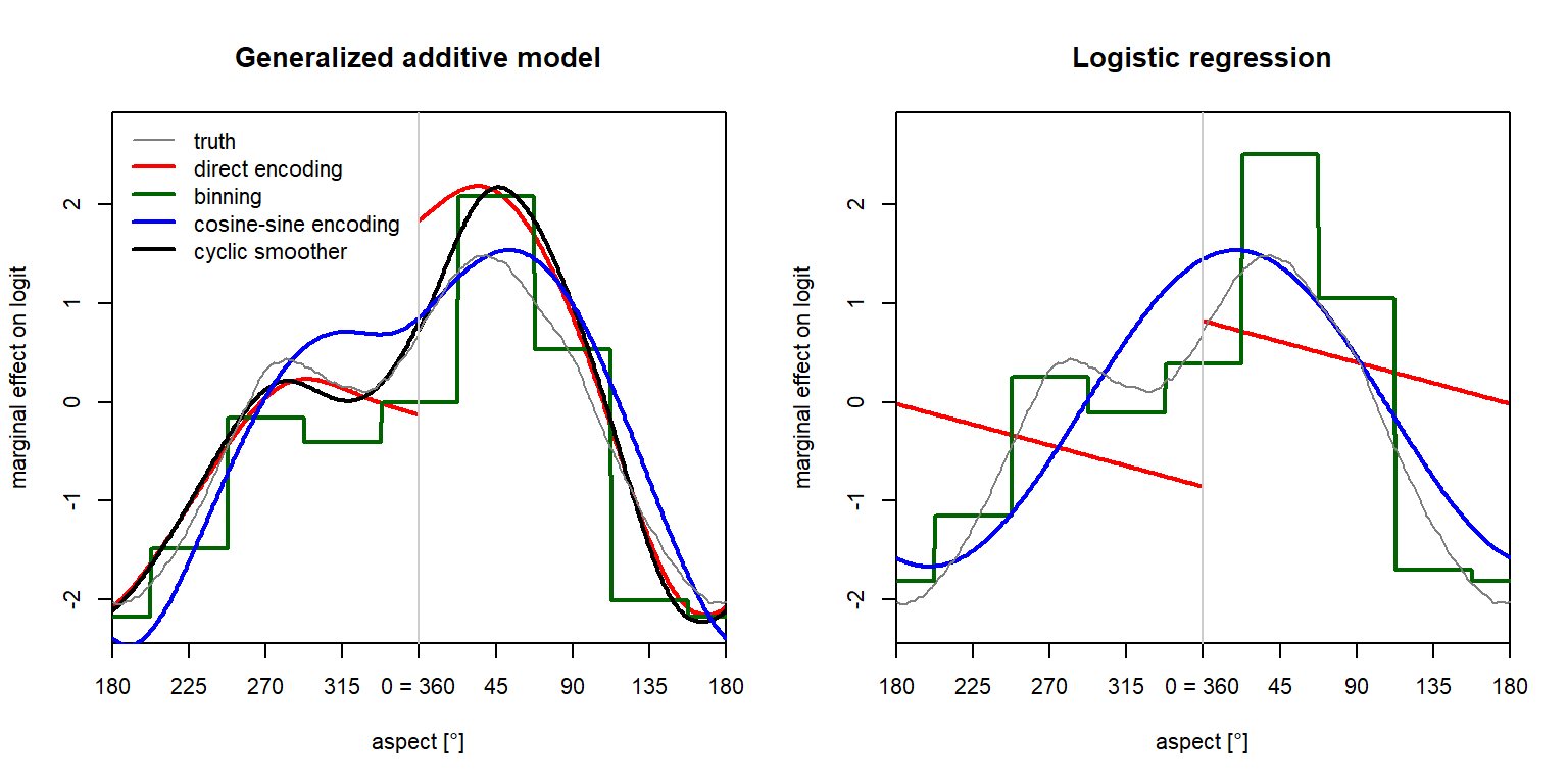
It turns out that the direct encoding results in a discontinuity at 0° in the effect of aspect on the predictions. The gap’s magnitude is about 2 on the logit scale, which means that the odds ($p/(1-p)$) change by a factor of about exp(2) = 7.4. This is not plausible at all, and it would result in erratic patterns in prediction maps.
In the GAM, the cyclic smoother and the cosine-sine encoding both produce reasonable approximations of the true curve, considering uncertainties due to random variability. Nevertheless, with cosine-sine encoding, the secondary peak is slightly shifted, which is a phenomenon I frequently observed in different simulation runs. Although the cyclic smoother does not decompose slope aspect into its cosine and sine, it is capable of modeling a nonlinear relationship that is continuous everywhere in the cycle.
In logistic regression, direct encoding also produces a gap, and the modeled relationship is not even strictly linear, as it has a breakpoint at 0° in our shifted plot. The GLM with cosine-sine encoding is unable to model the two peaks; this may not be a problem when datasets are small or slope aspect has little importance, but in general we may find this too limiting.
Binning the aspect variable results in a step function with eight levels. The effects associated with each aspect interval are only supported by the number of observations within that interval, which can be a limiting factor in many practical applications (but not in my simulated case study). While binned variables are easy to interpret, the step function results in implausible discontinuities in prediction maps.
The degrees of freedom associated with slope aspect are a good summary of how much flexibility the models deem necessary when modeling this relationship using different strategies:
| Model | Strategy | Degrees of freedom |
|---|---|---|
| GLM | Direct encoding | 1 |
| GLM | Binning | 7 |
| GLM | Cosine-sine encoding | 2 |
| GAM | Direct encoding | 5.14 |
| GAM | Binning | 7 |
| GAM | Cosine-sine encoding | 3.23 |
| GAM | Cyclic smoother | 4.75 |
What about more flexible ML techniques?
Next, I use the support vector machine (SVM) and random forest (RF) classifiers with direct and cosine-sine as well as binned encodings of slope aspect. Both models were tuned using 5-fold cross-validation; random forest uses trees to reduce artefacts.
Partial dependence plots display the marginal effects of predictors on the response in these non-additive models:
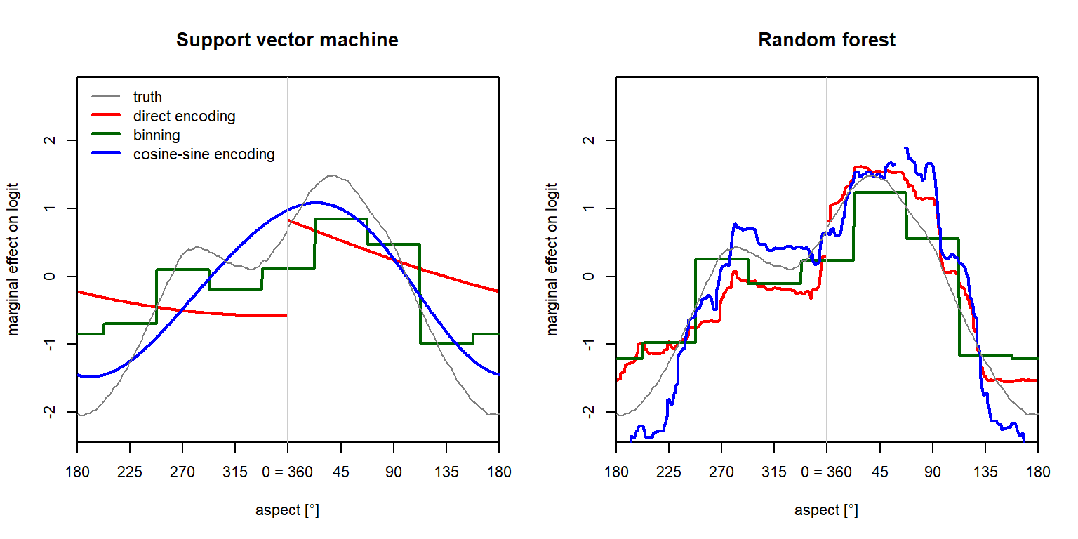
SVM exhibits the same problems we saw in logistic regression, but the cosine-sine encoding is certainly the better choice. Model shrinkage is very strong here, and therefore the relationships are strongly simplified.
RF shows the typical behaviour with fine step-like patterns and some artefacts in spite of the large number of trees used (2000). Focusing on the critical point at 0° = 360° aspect, there’s a relatively small jump in the RF with direct encoding of aspect, and no offset when using cosine-sine encoding. Nevertheless, the jump is not particularly remarkable compared to the usual variability in RF marginal effects.
Binning shows the expected step-function behaviour, which does not exploit the capabilities of SVM and RF to model more complex nonlinear relationships.
Overall, some ML models may be more sensitive to the peculiarities of directional variables, and we’d expect smooth models like SVM or artificial neural networks to benefit most strongly from cosine-sine encodings than tree-based models including boosting.
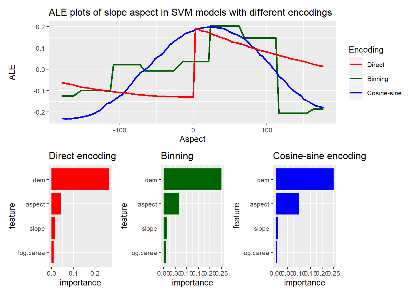
How can I obtain model diagnostics for aspect when using cosine-sine encoding?
If you are familiar with model diagnostics such as ALE plots and permutation-based variable importance (PVI) (e.g., Molnar 2019), you may wonder how these tools can be applied to visualize the overall importance of aspect – and not of its cosine and sine separately. The problem is that cosine and sine do not vary independently of each other. For example, a cosine of 1 can only be combined with a sine of 0 in order to obtain a valid point on the unit circle representing an angle in polar coordinates.
We can solve this by looking at the encoding-based models from the perspective of slope aspect itself.
We just need a wrapper function for the predict method that calculates the encoded features based on the input aspect values.
This wrapper function can be input into the function of the iml package for creating ALE plots and calculating permutation-based variable importance (Molnar, Bischl, and Casalicchio 2018).
By the way, this is a special case of the transformation approach I proposed recently to examine models in terms of features that aren’t even included in the model (Brenning 2021).
The following ALE plots and variable importances examine the marginal relationship between aspect and the response regardless of the chosen encoding:
Take-home message
So, what have learned?
- Never use slope aspect (and other cyclic variables) as a predictor without further ado.
- In a GAM, cyclic smoothers are the best way to include slope aspect.
- In general machine-learning models, use cosine-sine encoding to avoid artifacts.
- Avoid binning aspect; cosine-sine encoding and cyclic smoothers provide more flexibility with fewer degrees of freedom.
- If there’s a specific azimuth direction (or point in the cycle) where you expect the maximum or minimum, you can shift the aspect variable before calculating the (co)sine.
R Code
The R code for this analysis is available in Github.
References
Boeckli, L., A. Brenning, S. Gruber, and J. Noetzli. 2012. “A Statistical Approach to Modelling Permafrost Distribution in the European Alps or Similar Mountain Ranges.” The Cryosphere 6: 125–40. https://doi.org/10.5194/tc-6-125-2012.
Brenning, A. 2021. “Transforming Feature Space to Interpret Machine Learning Models.” http://arxiv.org/abs/2104.04295.
Brenning, A., M. Schwinn, A. P. Ruiz-Paez, and J. Muenchow. 2015. “Landslide Susceptibility Near Highways Is Increased by 1 Order of Magnitude in the Andes of Southern Ecuador, Loja Province.” Nat. Hazards Earth Syst. Sci. 15: 45–57. https://doi.org/10.5194/nhess-15-45-2015.
Brenning, A., and D. Trombotto. 2006. “Logistic Regression Modeling of Rock Glacier and Glacier Distribution: Topographic and Climatic Controls in the Semi-Arid Andes.” Geomorphology 81 (1-2): 141–54. https://doi.org/10.1016/j.geomorph.2006.04.003.
Deluigi, N., C. Lambiel, and M. Kanevski. 2017. “Data-Driven Mapping of the Potential Mountain Permafrost Distribution.” Science of the Total Environment 590-591: 370–80. https://doi.org/10.1016/j.scitotenv.2017.02.041.
London, I. 2016. “Encoding Cyclical Continuous Features - 24-Hour Time.” https://ianlondon.github.io/blog/encoding-cyclical-features-24hour-time/.
Meyer, H., C. Reudenbach, S. Wöllauer, and T. Nauss. 2019. “Importance of Spatial Predictor Variable Selection in Machine Learning Applications – Moving from Data Reproduction to Spatial Prediction.” Ecological Modelling 411: 108815. https://doi.org/10.1016/j.ecolmodel.2019.108815.
Molnar, C. 2019. Interpretable Machine Learning: A Guide for Making Black Box Models Explainable. https://christophm.github.io/interpretable-ml-book/.
Molnar, C., B. Bischl, and G. Casalicchio. 2018. “Iml: An R Package for Interpretable Machine Learning.” JOSS 3 (26): 786. https://doi.org/10.21105/joss.00786.
Stage, A. R. 1976. “An Expression for the Effect of Aspect, Slope, and Habitat Type on Tree Growth.” Forest Science 22: 457–60. https://doi.org/10.1093/forestscience/22.4.457.
Stage, A. R., and C. Salas. 2007. “Interactions of Elevation, Aspect, and Slope in Models of Forest Species Composition and Productivity.” Forest Science 53: 486–92.
Wood, S. N. 2017. Generalized Additive Models: An Introduction with R. CRC Press.